[Stata] Longitudinal Modeling with Fixed and Random Effects: xtreg
Understanding fixed and random effects
When working with panel data or longitudinal data, where you have multiple observations for the same individuals over time, it’s important to consider these effects. If not accounted for properly, these effects can lead to biased and inconsistent estimates. This is where fixed-effects and random-effects models come into play.
- Panel data, also known as longitudinal data, consists of observations on multiple entities (cross-sectional units) over time. These entities can be countries, firms, individuals, etc.
- Each entity is observed repeatedly across different time periods, resulting in a panel structure.
Unobserved individual-specific effects are factors or characteristics that are unique to each individual in a panel dataset but are not directly measured or included in the model. These effects can influence the dependent variable and may be correlated with the independent variables, leading to biased estimates if not accounted for properly.
Consider the relationship between patient adherence to treatment plans (X, measured through medication adherence rates) and health outcomes (Y) over several years. You have panel data for a group of patients.
In this case, the unobserved individual-specific effects could be factors such as:
- Patient Engagement: Some patients may be more engaged with their health management, leading to higher adherence rates and better health outcomes. Patient engagement is a personal trait that is challenging to measure and incorporate into the model.
- Socioeconomic Factors: A patient’s socioeconomic status, including income level and access to healthcare, might impact their health outcomes. These factors may not be fully captured in the dataset.
First, let’s consider a basic model for panel data:
Y_it = β_0 + β_1 * X_it + α_i + ε_it
Where:
- Y_it is the dependent variable for individual i at time t
- X_it is the independent variable for individual i at time t
- β_0 is the intercept
- β_1 is the coefficient for the independent variable
- α_i represents the unobserved individual-specific effects
- ε_it is the error term
The key question is: how should we treat the individual-specific effects (α_i)?
Fixed Effects Model: In the fixed effects model, we assume that α_i is correlated with the independent variables (X_it). This means that there are unobserved time-invariant factors that affect both the dependent variable and the independent variables. To remove the impact of these unobserved factors, the fixed effects model focuses on the within-individual variation by subtracting the individual means from each variable:
(Y_it - Y_i) = β_1 * (X_it - X_i) + (ε_it - ε_i)
If these unobserved effects are correlated with the independent variable (adherance), using a simple OLS regression would lead to biased estimates. The fixed effects model addresses this issue by focusing on the within-individual variation, effectively controlling for the unobserved time-invariant individual-specific effects. In the fixed effects model, the unobserved effects are captured by the individual-specific intercepts (α_i), which are eliminated by subtracting the individual means from each variable. This allows for consistent estimation of the relationship between X and Y, even in the presence of unobserved individual-specific effects. By doing this, the individual-specific effects (α_i) are eliminated, and we can obtain consistent estimates of β_1.
In an example of patient adherence, a fixed effect model is essential to control for omitted variables like “patient health literacy,” which is related to the predictor of healthcare access. There could be a systematic tendency for patients with better access to healthcare or higher-quality healthcare services to have higher health literacy, influencing both treatment adherence and health outcomes. Omitted variables like higher health literacy (correlated with better healthcare access) amplify the perceived impact of the predictor on the outcomes. The error linked to this omitted variable (patient’s health literacy) remains constant and is associated with the predictor (healthcare access), heightening the risk of a type one error.
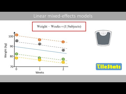
Fixed effect models fit multiple lines across individuals since they estimate the coefficients focusing on “within-individuals.”

Random Effects Model: In the random effects model, we assume that α_i is uncorrelated with the independent variables (X_it). This means that the unobserved individual-specific effects are random and not related to the independent variables.
In other words, if the unobserved individual-specific effects are not correlated with the independent variable, the random effects model can be used. In this case, the unobserved effects are treated as random variables and included in the error term, allowing for more efficient estimation.
In this case, we can include α_i in the error term:
Y_it = β_0 + β_1 * X_it + (α_i + ε_it)
The random effects model takes into account both the within-individual and between-individual variation, which can lead to more efficient estimates compared to the fixed effects model.
In the context of the patient adherence example, employing a random effects model allows for the examination of the variability across different healthcare environments or patient groups without assuming these effects are the same for every individual. This model recognizes that:
- Healthcare Environment Variability: Patients may access healthcare services from different environments (e.g., hospitals, clinics) that have unique characteristics affecting health outcomes. These characteristics could include the quality of care, patient-to-provider ratios, or available medical technologies. A random effects model can account for these unobserved environmental factors by assuming these effects are randomly distributed across the population.
- Genetic Predispositions: Patients have unique genetic backgrounds that may influence how they respond to treatment, affecting their health outcomes. While it’s challenging to measure and include every aspect of a patient’s genetic predisposition in the study, a random effects model allows for the assumption that these unobserved genetic factors vary randomly across individuals, influencing their response to treatment and overall health outcomes.
In essence, the random effects model is beneficial for acknowledging and incorporating the variability and heterogeneity inherent in patient populations and healthcare environments, without having to directly measure every possible influencing factor. The potential impact of unobserved individual-specific effects.
| Aspect | Fixed Effects (FE) | Random Effects (RE) |
|---|---|---|
| Definition | Represent constant parameters that apply to all individuals in the sample. | Capture variation across different subjects (individual-specific deviations). |
| Purpose | Used when we want to study the specific levels of a factor (e.g., treatment groups, time points). | Used when we want to account for individual variability in the data. |
| Estimation | Estimated directly using methods like least squares or maximum likelihood. | Not directly estimated; summarized by their variances and covariances. |
| Interpretation | Coefficients represent average effects across all individuals. | Variability in effects across different subjects (e.g., varying intercepts or slopes). |
| Example | We might investigate how the average reaction time changes with the number of days of sleep deprivation. The fixed effect coefficients would represent the overall trend across all subjects. | Now, let’s account for individual differences. Each subject has their own baseline reaction time and unique response to sleep deprivation. The random effect for subjects captures this variability. |
| Strengths | Simple interpretation, useful for specific comparisons. | Accounts for heterogeneity, generalizes to larger populations. |
| Limitations | Assumes all individuals are exchangeable, may not capture subject-specific variability. | Requires more complex modeling, may need larger sample sizes. |
You can also watch this video for a better understanding:
In this blog post, we’ll explore how to run and interpret these models using Stata and a sample dataset.
Step 1. Setting Up the Data:
First, let’s load a sample dataset in Stata. We’ll use the “nlswork” dataset, which contains panel data on young women’s labor force participation. To load the dataset, use the following command:
webuse nlswork, clearThe dataset includes variables such as:
- ln_wage: log of hourly wage (DV)
- union: union membership (IV)
- age: age in years (IV)
- grade: years of schooling (IV)
- not_smsa: does not live in SMSA (IV)
- south: lives in the south (IV)
Step 2. Running a Fixed Effects Model:
A fixed effects model allows you to control for time-invariant unobserved heterogeneity within individuals. To run a fixed effects model in Stata, use the “xtreg” command with the “fe” option. For example, let’s estimate the effect of union membership on wages:
xtreg ln_wage union age grade not_smsa south, fe
estimates store fixed // save estimates for hausman test
Interpreting the Fixed Effects Model: Coefficients indicate how much Y changes when X increases by one unit. Since the outcome is log-transformed here (ln_wage), you can interpret it as a percentage change. Please find this post by Stata to learn more.
- Union membership increases log wages by 0.10 within individuals over time, holding other factors constant (p < . 001).
- Each additional year of age increases wages by 0.015 within individuals (p < .001).
- The grade variable was omitted due to collinearity, meaning it does not vary within individuals over time.
- Living outside an SMSA decreases wages by 0.103, and living in the South decreases wages by 0.071 (-0.0709208) within individuals, which are both significant effects.
- The “F test that all u_i=0” tests the significance of individual fixed effects. A significant result suggests that fixed effects are needed.
- The “rho” value indicates the fraction of variance due to individual-specific effects (u_i): 71.1% of the variance is due to differences across individuals (rho).
the output provides the F-test result with the null hypothesis that all individual-specific intercepts are zero.
- If the null is accepted (p > .05), choose the pooled regression model;
- If rejected (p < .05), choose the fixed effects model.
[Advanced] Further, to determine if time-fixed effects significantly improve the model, we perform a joint F-test on all-year dummies:
xtreg ln_wage union age grade not_smsa south i.year, fe robust
testparm i.year
In this step, i.year adds year dummies to the model, capturing time fixed effects. testparm i.year tests if all coefficients for the year dummies are jointly equal to zero. A significant p-value (< 0.05) suggests that time fixed effects are necessary for the model.

Step 3. Running a Random Effects Model:
A random effects model assumes that the individual-specific effects are uncorrelated with the independent variables. To run a random effects model, use the “xtreg” command with the “re” option:
xtreg ln_wage union age grade not_smsa south, re
estimates store random // save estimates for hausman test
Interpreting the Random Effects Model: The coefficients represent the effects of the independent variables on log wages, accounting for both within-individual and between-individual variation.
Interpretation of the coefficients is tricky since they include both the within-entity and between-entity effects. The average effect of X over Y when X changes across time and between countries by one unit.
- Union membership is associated with 0.121 points higher log wages on log average between and within individuals. This is a larger effect than the fixed effects estimate.
- An additional year of age relates to 0.013 higher log wages on average, slightly smaller than the fixed effects estimate.
- Now, grade can be included since it varies across individuals. On average, an extra year of schooling is associated with 0.076 higher log wages.
- Not living in an SMSA relates to 0.138 lower log wages, and living in the South, with 0.093 lower log wages on average, has larger penalties than the within-effects from the fixed model.
- The “rho” value indicates the fraction of variance due to individual-specific effects (u_i): 58.9% of the wage variance is due to differences between individuals (rho).
- The “sigma_u” and “sigma_e” values represent the standard deviations of the individual-specific effects and the idiosyncratic error term, respectively.
xttest0After estimating the random effects model, you can perform the Breusch-Pagan LM test using xttest0 after the RE model estimation.
▶️The LM test assists in choosing between a random effects model and a standard OLS regression by testing the null hypothesis that there is no variation across entities, meaning there’s no significant difference between units, or in other words, no panel effect exists.

A significant p-value (Prob > chibar2 < 0.05) suggests the necessity of random effects.
Step 4. Choosing Between Fixed and Random Effects:
To decide between fixed effects and random effects, you can always use your purpose of study: What are you interested in? For example, if you are interested in the change within individuals, you can use a fixed-effects model. If you are interested in change across individuals, you can use the random effects model instead. Statistically, you can use the Hausman test. This test compares the coefficients from both models to determine whether the differences are systematic. If the test rejects the null hypothesis, it suggests that the fixed effects model is more appropriate, as there are likely omitted time-invariant variables that are correlated with the regressors.
To run the Hausman test, use the “hausman” command after running both fixed and random effects models:
hausman fixed random, sigmamore
In this case, the Hausman test yields a chi-square statistic of 173.99 with 4 degrees of freedom and a p-value of 0.0000 (p < .001). This means we reject the null hypothesis, indicating that the fixed effects model is more appropriate for this data. This implies that there are likely omitted time-invariant variables that are correlated with the regressors, making the random effects model inconsistent.
Looking at the coefficient differences:
- For union, age, not living in an SMSA, and living in the South, the fixed effects estimates are smaller in magnitude than the random effects estimates.
- The standard errors of these differences (sqrt(diag(V_b-V_B))) are relatively small, suggesting these differences are precisely estimated.
In conclusion, based on the Hausman test results, the fixed effects model is preferred for this analysis, as it allows for consistent estimation in the presence of omitted time-invariant variables that are correlated with the included regressors.
Step 5. Model Diagnostics and Tests
(1) Evaluating Cross-Sectional Dependence
Baltagi (2007) highlights that cross-sectional dependence poses a challenge in macro panels characterized by long-term time series data spanning 20-30 years.
Cross-Sectional Dependence:
- This issue arises when residuals among entities are interconnected, assuming initially that residuals are not interrelated.
- The presence of cross-sectional dependence affects estimation and inference in panel-data models.
- Efficiency: Standard fixed-effects (FE) and random-effects (RE) estimators remain consistent but become inefficient when cross-sectional dependence exists.
- Biased Standard Errors: The estimated standard errors are biased due to the correlation among residuals.
- Researchers need to account for cross-sectional dependence to obtain reliable parameter estimates and valid statistical tests.
Example of Cross-sectional dependence
- Scenario: Imagine a study examining the prevalence of mental health disorders (such as anxiety and depression) among different age groups in a community.
- Cross-Sectional Dependence:
- The mental health outcomes of individuals within the same family might be correlated due to shared genetic factors or common environmental influences.
- Social interactions (e.g., support networks, stigma) could lead to similar mental health outcomes among friends or neighbors.
- Researchers need to account for these dependencies when analyzing mental health data.
Testing for Cross-Sectional Dependence
Option A. Baltagi’s B-P/LM Test of Independence: The null hypothesis in the B-P/LM test of independence is that residuals across entities are not correlated.
xtreg ln_wage union age grade not_smsa south, fe
xttest2
Significant results (Pr < 0.05) indicate cross-sectional dependence.
Option B. Pasaran CD Test: The Pasaran CD test evaluates the presence of cross-sectional dependence by examining the correlation of residuals across entities, with its null hypothesis positing no such correlation exists.
ssc install xtcsd
xtcsd, pesaran abs
A significant p-value (Pr < 0.05) confirms cross-sectional dependence.
Cross-Sectional Dependence Correction: If cross-sectional dependence is present, consider using Driscoll and Kraay standard errors with the command xtscc.
ssc install xtscc xtscc ln_wage union age grade not_smsa south, fe(2) Checking for Heteroskedasticity
Modified Wald Test for Groupwise Heteroskedasticity: Use xttest3 after estimating the FE model to test for heteroskedasticity.
xttest3
- Rejecting the null hypothesis (Prob > chi2 < 0.05) indicates heteroskedasticity.
Fixed-Effects Model with Robust Standard Errors: To address heteroskedasticity, you can estimate the model using the FE estimator with robust standard errors.
xtreg ln_wage union age grade not_smsa south, fe robust(3) Testing for Serial Correlation
Serial correlation tests are particularly relevant for macro panel datasets that span long periods, typically 20-30 years or more (see here to learn more). They are less of a concern in micro panels, which cover only a few years. Serial correlation leads to underestimation of the standard errors for coefficients and inflated R-squared values, potentially misleading about the model’s fit.
Serial Correlation Test: After estimating the FE model, use xtserial to test for first-order autocorrelation.
ssc install xtserial
xtreg ln_wage union age grade not_smsa south, fe robust
xtserial ln_wage union age grade not_smsa south
- A significant p-value (Prob > F < 0.05) suggests the presence of serial correlation.
Reference
Five ways to detect correlation in panels (stata.com)
