[Stata] Multilevel Mixed-Effects Linear Regression: mixed
Understanding Fixed Effects, Random Effects, and Mixed Effects

1) Fixed Effects Models: In fixed effects models, the effects of the independent variables are assumed to be constant across all groups or levels in the data.
- The model estimates a single coefficient for each independent variable, which applies universally across all entities (e.g., individuals, schools, regions).
- This approach is used when the interest is in analyzing the impact of variables within an entity over time or the differences in a variable across entities, assuming that every entity has its unique intercept.
- They control for all time-invariant differences between the entities, thus eliminating omitted variable bias due to unobserved heterogeneity when the omitted variable does not vary over time.
- The model focuses on the within-entity variation over time, disregarding the between-entity variation.
- Fixed effects models are particularly useful when the goal is to understand the causal relationships between variables.
Random Effects Models: Random effects models, on the other hand, assume that the variation across entities can be captured in a random component of the model.
- This approach is used when there is reason to believe that differences across entities (or time periods) have some influence on the dependent variable, but these differences are not the primary focus of the study.
- In random effects models, besides estimating a single coefficient for each independent variable (like in fixed effects models), the model also estimates the variance components associated with the random effects.
- They are more efficient than fixed effects models if the random effects assumption holds (i.e., the entity’s error term is not correlated with the predictors).
- The model considers both within-entity and between-entity variation, providing a broader understanding of the data.
- Random effects models are suitable when the interest lies in understanding the impact of variables that vary between entities, assuming that entities are a random sample from a larger population.
Mixed-Effects Models: Mixed-effects models (or multilevel models) combine fixed and random effects. They allow for coefficients to vary across groups for some variables (random slopes) and to be constant for others (fixed effects).
- This flexibility makes mixed-effects models particularly powerful for analyzing hierarchical or nested data structures, such as students within schools or repeated measures within individuals.

The choice between fixed effects, random effects, and mixed-effects models should be guided by your research question and the structure of your data:
- Fixed Effects Models are preferred when you believe that something within the individual may both influence the predictor variables and also be correlated with the outcome, and you want to control for all invariant characteristics of the individuals.
- Random Effects Models are used when you assume that the individual-specific effects are random and not correlated with the independent variables. They are more efficient than fixed effects models if this assumption holds.
- Mixed-Effects Models are chosen when you have data that is hierarchical or nested and you want to allow for varying effects at different levels of the hierarchy — multilevel modeling!
Remember to perform diagnostic tests, such as the Hausman test for choosing between fixed and random effects, and consider model fit statistics when comparing mixed-effects model specifications.
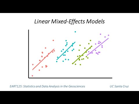
Please refer to the following video for more understanding of the mixed effects.
Stata Commands for Multilevel Modeling

mixed: linear multilevel model (renamed fromxtmixedfrom Stata version 14. So they are identical commands)
If you would love to use the outcomes for generalized linear modeling, you can use the following commands instead of mixed.
melogit: Multilevel mixed-effects for binary responses (logistic regression)meologit: mixed-effects logistic models for ordered responses (ordinal logit)mepoisson: Multilevel mixed-effects Poisson regressionmbenreg: mixed-effects negative binomial models to count datameglm: multi-level mixed-effects generalized linear model
Step 1. Preparing the Data
For multilevel modeling, ensure your data is properly structured for the analysis. Now, let’s look at the example. We’ll use the nlsw88 dataset for this purpose, as it contains hierarchical data suitable for demonstrating both fixed effects and random slopes.
webuse nlsw88, clear
describe
Step 2. Model without Random Slope
Assuming industry is the grouping variable (level-2) and individuals are level-1 units. We’ll start by fitting a basic multilevel model with random intercepts for the groups (industries) without random slopes. Let’s say we’re interested in how wage is affected by age and education:
mixed wage age i.collgrad || industry:, variance This command tells Stata to fit a model where wage is modeled as a function of age and education, with a random intercept for each industry.
After running the mixed command, Stata will output several pieces of information, including estimates for fixed effects, variance components for random effects, and model fit statistics. Here’s a brief on what to look for:
- Fixed effects: Coefficients represent the average effect of each predictor on the outcome variable.
- Random effects: Variance components indicate how much variation there is in the intercepts and slopes across groups.
- Model fit: Look at statistics like the -2 Log likelihood to compare models.

This model estimates the effects of age and collgrad (college graduate status) on wage, with random intercepts for industry. The results are based on maximum likelihood estimation (MLE) by default in Stata.
Determining the statistical significance of random effects in mixed-effects models is less straightforward than assessing fixed effects because standard significance tests (like t-tests for fixed effects) do not directly apply. One primary method is to look at the confidence intervals for the variance components of the random effects. If the 95% confidence interval for a variance component does not include zero, it suggests that there is significant variability captured by that random effect.
Further, the LR test compares the log-likelihoods of two nested models (one with and one without the random effect). A significant result (usually p < 0.05) suggests that the model with the random effect fits the data significantly better than the model without it, indicating the significance of the random effect.
- Fixed Effects:
age: The coefficient is -0.052, not statistically significant (p = 0.161), suggesting no clear effect of age on wage across industries.collgrad(College grad): The coefficient is 3.844, significant (p < 0.001), indicating that college graduates earn, on average, 3.844 units more than non-graduates across all industries.
- Random Effects:
var(_cons)withinindustry: The variance is 3.838, suggesting differences in the baseline wage across industries.var(Residual): The residual variance is 28.876, representing the within-industry wage variation not explained by the model.
- Model Fit:
- The LR test vs. a linear model is significant (p < 0.001), justifying the use of random effects. This indicates that the improvement in model fit with the inclusion of random effects is statistically significant. In other words, the random effects (such as random intercepts or random slopes) capture significant variability in the data that is not explained by the fixed effects alone.
Step 3. Adding Random Slopes
To allow for random slopes, you must specify which variable(s) you want to allow to vary by group. For instance, if we think the effect of education on wage might vary across industries, we add a random slope:
mixed wage age i.collgrad || industry: i.collgrad, varianceFixed Effects: In our model, age and education are fixed effects. This means we assume these effects (the relationship between these predictors and wage) are consistent across all industries.
Random Effects: The random intercept for industry allows the baseline wage to vary across industries. Adding a random slope for education by industry lets the effect of education on wage vary across industries.

This model allows the effect of collgrad on wage to vary across industry.
- Fixed Effects:
age: Similar to the first model, the effect of age is not significant (p = 0.153).collgrad(College grad): The coefficient is 3.850, still significant (p < 0.001), with a similar interpretation but a larger standard error due to the introduction of random slopes.
- Random Effects:
var(1.collgrad): The variance of the slope forcollgradacross industries is 1.312, indicating variability in the wage premium for college graduates across industries.var(_cons): The variance in the intercept has slightly increased to 3.911, reflecting variations in baseline wages.var(Residual): Slightly reduced to 28.754, indicating a small change in the unexplained within-industry wage variation.
- Model Fit and Comparison:
- Log likelihood: -6934.654 suggests a slightly better fit than the model without random slopes, as indicated by a smaller (more negative) log likelihood.
- The LR test vs. the linear model remains significant, and the introduction of random slopes for
collgraddoes not change the overall conclusion that the model with random effects is preferred over a simple linear regression.
Options
In the context of Stata’s mixed command for multilevel modeling, the variance and cov(unstructured) options define different structures for the variance-covariance matrix of the random effects. The choice between these two options depends on your hypothesis about the random effects. If you believe they are correlated, cov(unstructured) would be more appropriate.
- Variance (
variance): This option specifies that the random effects have a diagonal covariance structure. It means that each random effect has its own variance, but all covariances between random effects are assumed to be zero. In other words, it assumes that the random effects are uncorrelated. - Unstructured Covariance (
cov(unstructured)): This option allows for the estimation of all variances and covariances without imposing any structure. It means that each random effect has its own variance, and every possible covariance between random effects is also estimated. This results in a full variance-covariance matrix and does not assume that the random effects are uncorrelated.
Reference
- stata.com/features/overview/multilevel-mixed-effects-models/
- Multilevel/ Mixed Effects Models: A Brief Overview (nd.edu)
- Module 5: Introduction to Multilevel Modelling (bristol.ac.uk)
- https://www.princeton.edu/~otorres/Multilevel101.pdf
- https://grodri.github.io/multilevel/pop510slides1.pdf
- How can I run multilevel models in Stata? (Stata 11) | Stata FAQ (ucla.edu)
- How can I convert a multilevel model to a mixed model? | Stata FAQ (ucla.edu)
- Introduction to Multilevel Modeling by Kreft and de Leeuw Chapter 4: Analyses | Stata Textbook Examples (ucla.edu)
- How can I perform mediation with multilevel data? (Method 1) | Stata FAQ (ucla.edu)
- How can I perform mediation with multilevel data? (Method 2) | Stata FAQ (ucla.edu)
- Multilevel generalized linear models | Stata
- The Stata Blog » Multilevel linear models in Stata, part 1: Components of variance
- Stata Bookstore: Multilevel and Longitudinal Modeling Using Stata, Fourth Edition
- Tricks of the Trade: Getting the most out of xtmixed (stata.com)
- Multilevel mixed models for binary and count responses (stata.com)
- Module 7: Multilevel Models for Binary Responses
- Multilevel Models with Binary and other Noncontinuous Dependent Variables (pxu.edu)
