[Stata] Logistic Regression: Model Fitting, Diagnosis, and Predicted Probabilites

Logistic regression is a statistical method for modeling binary outcomes, such as yes/no, success/failure, or alive/dead. It allows us to estimate the probability of an event occurring as a function of one or more predictors, such as age, gender, income, or education. In this post, we will use Stata to perform a logistic regression analysis on the nhanes2 webuse dataset, which contains data from the second National Health and Nutrition Examination Survey (NHANES II) conducted in 1976-1980. We will use the variable highbp, which indicates whether the respondent has high blood pressure as our binary outcome variable, and the variables age, sex, race, and bmi (body mass index) as our predictors. We will also compare the results of the logit model with those of the probit model, which is another common way of modeling binary outcomes.

Data Preparation

Before we run the logistic regression, we need to load the nhanes2 webuse dataset and do some data preparation. We can use the webuse command to load the dataset from the Stata website. We also can use the describe command to see the variables and their labels in the dataset.

webuse nhanes2
describe

We can see that the dataset has 10,351 observations and 58 variables. The variable highbp is coded as 1 for respondents who have high blood pressure and 0 for those who do not. The variables age, sex, race, and bmi are the predictors (independent variables) we are interested in.

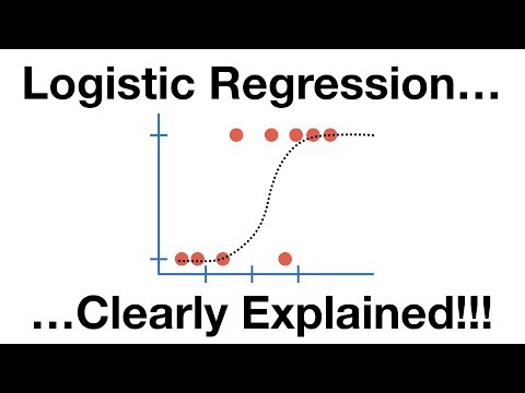
Step 1. Scatter Plot of X and Y

To explore the association between predictor and outcome, we can use the scatter command to graph one of our continuous predictors, such as bmi, against the binary outcome, highbp. We can also add the option jitter(3) to add some random noise to the vertical position of the points, so that they do not overlap too much. Jitter number more than 10 would be too much random noise, so please keep it under 10. Here is the command and the resulting graph:

scatter highbp bmi, jitter(3)

We can interpret the scatter plot as follows:

• The scatter plot shows the relationship between body mass index (bmi) and high blood pressure (highbp) for the nhanes2 webuse dataset.
• The horizontal axis represents the bmi, which is a measure of body fat based on weight and height. The vertical axis represents the highbp, which is a binary variable indicating whether the respondent has high blood pressure or not.
• The scatter plot suggests that there is a positive association between bmi and highbp, meaning that higher bmi is associated with higher probability of having high blood pressure. 
• However, the scatter plot also shows that there is a lot of variation and overlap in the data, meaning that bmi alone is not a very good predictor of highbp. There are many respondents who have high bmi but do not have high blood pressure, and vice versa. Therefore, we need to use other predictors and a logistic regression model to account for the complexity of the data.

What happens if we fit binary outcomes with LPM?

reg highbp age bmi i.sex i.race
avplots

For your information, rvfplot, avplots are concept related to LPM bu not relevant to logistic regressions.

Step 2. Fitting Logit Model with One Predictor

Then, we can proceed to use the logit command to regress our binary outcome variable, highbp, on one of our predictors, such as bmi. The logit command fits a logistic regression model, which estimates the log odds of the outcome as a linear function of the predictors. Here is the command and the output:

logit highbp bmi

The output shows the results of the logistic regression of high blood pressure (highbp) on body mass index (bmi) for the nhanes2 webuse dataset. We can interpret the output as follows. However, we never interpret coefficients/log odds in publishable papers. So, we need to stick with interpreting ORs.

• The coefficient of bmi is 0.149, which means that for every one unit increase in bmi, the log odds of having hypertension increase by 0.149, holding other variables constant. This implies that higher bmi is associated with higher probability of having high blood pressure, as we saw in the scatter plot.
• The standard errors of the coefficients are the estimated standard deviations of the sampling distributions of the coefficients. They measure the precision of the estimates. Smaller standard errors mean more precise estimates.
• The z-statistics are the ratios of the coefficients to their standard errors. They measure the significance of the coefficients. Larger z-statistics (in absolute value) mean more significant coefficients.
• The p-values are the probabilities of obtaining the coefficients (or more extreme values) by chance, if the null hypothesis of no effect is true. They measure the evidence against the null hypothesis. Smaller p-values mean more evidence against the null hypothesis.
• The 95% confidence intervals are the ranges of values that contain the true coefficients with 95% probability. They measure the uncertainty of the estimates. Narrower confidence intervals mean less uncertainty.
• The LR chi2(1) statistic is the likelihood ratio chi-square test of the overall fit of the model. It compares the log likelihood of the model with the log likelihood of the null model (which has only the constant term). It measures how much the model improves the fit compared to the null model. Larger LR chi2 statistics mean better fit.
• The Prob > chi2 is the p-value of the LR chi2 test. It measures the evidence against the null hypothesis that the model does not fit better than the null model. Smaller Prob > chi2 values mean more evidence against the null hypothesis.
• The log likelihood is the value of the log likelihood function at the estimated coefficients. It measures how well the model predicts the observed outcomes. Higher log likelihood values mean better prediction.
• The pseudo R2 is a measure of the proportion of variation in the outcome that is explained by the model. It is analogous to the R2 in linear regression, and higher pseudo R2 values mean more explanation.

Step 3. Residuals Plot of predictor and outcome

Then, we need to obtain the residuals from the logit model and plot them against the predictor, bmi. The residuals are the differences between the observed and predicted outcomes. They measure how well the model fits the data. We can use the predict command with the option residual to generate a new variable called resid that contains the residuals. We can then use the scatter command to graph the residuals against bmi. Here is the command and the resulting graph:

predict resid, residual
scatter resid bmi

We can interpret the residuals plot as follows:

• The residuals plot shows the relationship between the residuals and the body mass index (bmi) for the logit model of hypertension (highbp) on bmi.
• The horizontal axis represents the bmi, and the vertical axis represents the residuals. The points are colored by the observed values of highbp.
• The residuals plot shows that the logit model does not fit the data very well, as there is a clear pattern in the residuals. The residuals tend to be positive for low values of bmi and negative for high values of bmi, meaning that the model underpredicts the probability of hypertension for low bmi and overpredicts it for high bmi. This suggests that the logit model is too simple and linear to capture the nonlinear and complex relationship between bmi and highbp.
• The residuals plot also shows that there are some outliers in the data, such as the points with very high or very low bmi and large residuals. These are the cases where the model fails to predict the outcome correctly. For example, there are some respondents who have very low bmi but have hypertension, and some who have very high bmi but do not have hypertension. These outliers may have other factors that affect their blood pressure, such as genetics, lifestyle, or medication. Therefore, we need to include more predictors and a more flexible model to account for these factors.

Step 4. Logit Model with Multiple Predictors

For the next step, we need to use the logit command to regress our binary outcome variable, highbp, on all of our predictors, age, sex, race, and bmi. This will allow us to control for the effects of other factors that may influence the probability of having hypertension, and to test the significance of each predictor. Here is the command and the output:

logit highbp age i.sex i.race bmi

We can interpret the output as follows:

• The output shows the results of the logistic regression of hypertension (highbp) on age, sex, race, and body mass index (bmi) for the nhanes2 webuse dataset.
• The other statistics are similar to those in the previous model, except that they are based on the new model with multiple predictors. The LR chi2(5) statistic is much larger than the LR chi2(1) statistic, indicating that the model with multiple predictors fits the data much better than the model with only one predictor. The pseudo R2 is also higher, indicating that the model with multiple predictors explains more variation in the outcome than the model with only one predictor.

🔥What is the difference between the commands logit and logistic in Stata?

The logit command fits a logistic regression model and returns the coefficients by default. The logistic command is an alternative to logit. It displays estimates as odds ratios. You can also get the odds ratio by using logit command with or option.

• Coefficients: The raw coefficients (log odds) indicate the change in log odds associated with a one-unit increase in the predictor. Exponentiating these coefficients gives the odds ratio.
• Odds Ratio (OR): The exponentiated coefficient for each predictor represents the odds ratio.
  • An odds ratio (OR) is a measure of the association between a variable and an event. It tells you how the odds of the event change when the variable changes.
    • For example, an OR of 2 means that the odds of the event are twice as high when the variable is present than when it is absent.
    • An OR of 0.5 means that the odds of the event are half as high when the variable is present than when it is absent.
    • An OR of 1 means that the odds of the event are the same regardless of the variable.
  • For example, if the OR for age is 1.04, which means that for every one-unit increase in age, the odds of hypertension increase by 4%.

More Examples of Interpretation

Continuous Predictor

• A one-unit increase in age is associated with a 4% increase in the odds (OR = 1.05, 95% CI: 1.04, 1.05, p < 0.001).
• A one-unit increase in age has, on average, 1.04 times the odds of hypertension.
• A one-unit increase in age is associated with greater odds of hypertension by a factor of 1.04.
• A one-unit increase in age is associated with 4% greater (or higher) odds of hypertension.

Nominal Predictor

Please don’t forget to mention the reference group here!

• Being female is associated with a 39% decrease in the odds compared to males (OR = 0.62, 95% CI: 0.56, 0.62, p < 0.001).
• Women have 0.61 times the odds of hypertension compared to men.
• Women have lower odds of hypertension than men by a factor of 0.61.
• Women have 39% less odds of hypertension than men.

⚠️ You need to use the wording appropriate for your own dataset. For example, if your sample is about the youths, you can say black youths have a 44% increase in the odds compared to White counterparts.

⚠️ You need to be careful in interpreting the odds ratio as “likelihood” since the statistics use the term “likelihood” in different contexts (e.g., maximum likelihood estimator).

🧱Interpretation of odds ratio

To interpret an odds ratio, you can use the following guidelines:

• If the OR is greater than 1, it means that the variable is associated with higher odds of the event.
• If the OR is less than 1, it means that the variable is associated with lower odds of the event.
• If the OR is equal to 1, it means that the variable is not associated with the event at all.

You can also express the OR as a percentage increase or decrease in the odds of the event. To do this, you can use the formula:

Percentage change=(OR−1)×100%

For example, an OR of 1.5 means that the odds of the event are increased by 50% when the variable is present. An OR of 0.8 means that the odds of the event are decreased by 20% when the variable is present.

[Optional] Probit Model with Multiple Predictors

To run the probit model, we need to use the probit command to regress our binary outcome variable, hyperten, on all of our predictors, age, sex, race, and bmi. The probit command fits a probit regression model, which is similar to the logit model, but it assumes that the error term follows a standard normal distribution instead of a logistic distribution. Here is the command and the output:

probit highbp age i.sex i.race bmi

We can interpret the output as follows:

• The output shows the results of the probit regression of hypertension (highbp) on age, sex, race, and body mass index (bmi) for the nhanes2 webuse dataset.
• The other statistics are similar to those in the logit model, except that they are based on the probit model with multiple predictors. The pseudo R2 is also the same, indicating that the model with multiple predictors explains the same amount of variation in the outcome as the logit model.

To save the results of the logit and probit models side-by-side, you can use the following command.

logit highbp age i.sex i.race bmi
estimates store logit
probit highbp age i.sex i.race bmi
estimates store probit

estimates table logit probit, b(%9.3f) t varlabel

Step 5. Checking for specification errors using the linktest command

You need to run the command after estimating your logistic regression mode. You can run linktest right after logit command.

logit highbp age i.sex i.race bmi
linktest

In the results, linear predicted value (_hat) should be significant (p < .05) while linear predicted value squared (_hatsq) should not be significant (p > .05). If it is significant, there is probably an omitted variable (in my example). Please remember that this test does not mean that my model is correctly specified, only that it fits well. Moreover, do not let your statistical methods drive your methods- your expertise and knowledge of the literature should 🙂

You can also learn more about logistic regression diagnostics using link test here:

Lesson 3 Logistic Regression Diagnostics (ucla.edu)

linktest – Stata Help – Reed College

Step 6. Comparing model fits across models: lrtest and fitstat

Then, we’ll explore the process of comparing model fits across logistic regression models in Stata, using the lrtest (Likelihood Ratio test) and fitstat commands. This step is crucial when you’re trying to determine the necessity of certain variables in your model, aiming to strike a balance between model complexity and explanatory power — for the Parsimonious Model.

For this purpose, we can compare the reduced model and the full model. After running an initial logistic regression model including all these variables, we hypothesize that the bmi might be unrelated to bmi outcome. To test this hypothesis, we compare two models: a full model including the bmi variable and a reduced model excluding it.

First, we run a logistic regression including all variables of interest and then save it as estimates (full). Then, we can run another model without bmi variable, and then save it as estimates (reduced).

logit highbp age i.sex i.race bmi
estimates store full

logit highbp age i.sex i.race 
estimates store reduced

To compare the fit of the full model against the reduced model, we can use two approaches:

• Fitstat: This provides a variety of statistics to assess model fit. Although not explicitly shown here, invoking fitstat after running each model would give us insights into how well each model explains the data. Generally, if the reduced model fits significantly worse, this suggests that the excluded variable(s) contributed meaningful information.

logit highbp age i.sex i.race bmi
fitstat, saving(full)

logit highbp age i.sex i.race 
fitstat, saving(redu)

fitstat, using(full) saving(redu) // compare model 

The criteria we use — the smaller AIC / BIC indicate the better model fit. The results here are conflicting: the LR test is significant (= current model is better), and AIC is smaller in the current model. However, the BIC is smaller in the saved model.

• Likelihood Ratio Test (LR Test): The LR test compares the likelihood of the full model against the reduced model, testing the null hypothesis that the models fit the data equally well. A significant result would indicate that the full model (including child’s temperament) provides a significantly better fit to the data.

lrtest full reduced 

🔥 Interpretation: The LR test compares the likelihood of the full model against the reduced model, testing the null hypothesis that the models fit the data equally well. A significant result would indicate that the full model (including bmi – additional variable) provides a significantly better fit to the data.

Reference

journalfeed.org/article-a-day/2018/idiots-guide-to-odds-ratios/