[Stata] Examining outliers or high-leverage observations using predict command

In statistical analysis, particularly in regression models, identifying outliers and high-leverage observations is crucial for ensuring the accuracy and reliability of your findings. Outliers can significantly impact the results of a regression analysis, leading to misleading conclusions. Stata provides a robust toolkit for diagnosing and examining these observations through the predict command followed by various options. In this blog post, we’ll explore how to use these tools to identify and examine outliers or high-leverage observations in your dataset.

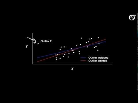
This is the best video to my knowledge to understand the concepts of outliers, high leverage points, and influence in regression.

Understanding Predict Command Options

The predict command in Stata, when used after fitting a regression model, can generate several types of residuals and diagnostic measures that are useful for identifying outliers and influential observations. Here’s a quick overview of the options we’ll discuss:

• pcont: Predicted values from the model (without any option)
• Residuals (resid): which are the differences between observed and predicted values.
• Standardized residuals (rstd): the standardized difference between the observed frequency and the predicted frequency, which are the residuals divided by their standard deviation, making it easier to identify outliers.
• Deviance residual (dev): the disagreement between the maxima of the observed and the fitted log likelihood functions. useful for logistic regression models to identify poorly predicted observations.
• Pregibon leverage (hat): observations with unusual predictor values that may overly influence the model fit.

Step 1: Generate Diagnostic Measures

After fitting your regression model, use the predict command with different options to generate the measures needed for diagnostic checks:

webuse nhanes2
logit highbp age i.race i.sex bmi

predict pcont // obtain predicted values 
predict resid, resid // obtain the (unstandardized) Pearson residual
predict rstd, rstandard // obtain the standardized Pearson residual
predict rdev, dev // obtain the deviance residual
predict rhat, hat // obtain the Pregibon leverage

These commands create new variables in your dataset: predicted values (pcont), residuals (resid), standardized residuals (rstd), deviance residuals (rdev), and Pregibon leverage values (rhat).

General rules:
1) standardized residuals > |2| = problematic
2) deviances > |2| = problematic
3) pregibon leverages > |2x the mean pregibon leverage| = problematic

Some people use the criteria of |3| instead of |2| for standardized residuals and deviances. You might need to provide the rationale such as 1) small sample size and 2) modeling issue – too few predictors, omitted variables.

Step 2: Visualizing Diagnostics

Visual inspection of these diagnostics can be highly informative. Scatter plots help visualize the relationship between diagnostic measures and other variables, including the predicted values or the observations’ index number (which can help identify specific problematic observations).

• Scatter Plot of Standardized Residuals:

scatter rstd sampl, mlab(sampl)
// sampl should be id in your dataset 

This plot helps identify outliers in your residuals. Observations with standardized residuals greater than 2 or less than -2 are typically considered outliers. The scatter plot of standardized Pearson residuals suggests that the majority of residuals fall within -2 and 2 standard deviations.

• Listing Observations with Extreme Standardized Residuals:

list sampl resid rstd if rstd > 2.58 | rstd < -2.58

This command lists observations with standardized residuals greater than 2.58 or less than -2.58, often considered as having extreme residuals.

Step 3: Examining Deviance Residuals and Leverage

For logistic regression models, deviance residuals (rdev) and leverage values (rhat) are particularly useful:

• Scatter Plot of Deviance Residuals:

  scatter rdev sampl, mlab(sampl)

Identifies observations with poor fit in logistic regression models. The scatter plot illustrates a small deviance as the majority of residuals are between -2 and 2 standard deviations.

• Scatter Plot of Leverage Values:

scatter rhat sampl, mlab(sampl)

High leverage points are observations with unusual combinations of predictor values that can overly influence the model’s estimation.

We can see what the mean leverage is in the sample:

sum rhat, detail

To calculate the threshold, multiply the mean leverage by two, which is 0.0006*2 = 0.0012. To identify concerning cases, look for values that are >2 on rstand and dev, and >twice the mean leverage.

Resource

Lesson 3 Logistic Regression Diagnostics (ucla.edu)

9.3 – Identifying Outliers (Unusual Y Values) | STAT 462 (psu.edu)