[Stata] One-sample/two-sample T-test (ttest, robvar, and esize)

T-test is a statistical method that compares the means of two groups or samples. It can be used to test hypotheses about the difference between the means, or to measure the effect size of the difference. In this blog post, I will show you how to run different types of t-tests in Stata.

Example: NHANES II data

The webuse nhanes2 dataset contains data from the National Health and Nutrition Examination Survey (NHANES) II, conducted by the National Center for Health Statistics (NCHS) from 1976 to 1980. It has information on 10,351 individuals, including their demographic characteristics, health status, and laboratory results. You can load the dataset in Stata by typing:

webuse nhanes2

One-sample t-test: t-test with a specific number

One type of t-test is to compare the mean of a variable with a specific number. For example, we can test whether the mean systolic blood pressure (bpsystol) in the dataset is equal to 120 mmHg, which is considered normal. To do this, we can use the ttest command with the == option:

ttest var1 == 120

The output shows that the mean bpsystol in the dataset is 130.88 mmHg, which is significantly different from 120 mmHg (p < 0.001).

T-test for Independent Samples

Step 1. Test equality of variance: robvar

The first step for an independent sample t-test is to test the equality of variance (i.e. homoscedasticity). You can use robvar for this. The robvar command performs Levene’s test, which is a way to test the equality of variances. The output of this command will show the summary statistics for each group and the combined group, as well as the test statistic and p-value for three versions of the test: centered at the mean (W0), centered at the median (W50), and centered using a 10% trimmed mean (W10).

robvar var1, by(groupvar)

To interpret the output, you can look at the p-value for each version of Levene’s test. If any p-value is less than 0.05, you can reject the null hypothesis (i.e., There is equal variance across groups) and accept the alternative hypothesis (i.e., there is a statistically significant difference in the variances between the groups). In other words, to ensure the assumptions of homoscedasticity, we want to accept the null hypothesis (i.e., equal variance), which means the p-value is non-significant.

** Note that Levene’s test is more robust to non-normality than the variance ratio test (sdtest), so it is recommended to use Levene’s test instead of sdtest, in most cases. You can see the W0 by default (centered at the mean). In the example, we have a significant p-value (p<0.001) at W0, so we have to add unequal option for the t-test.

• p > 0.05 : variances are equal (accept null hypothesis)
• p < 0.05 : variances are unequal (accept alternative hypothesis)

Learn more here: multiple comparisons – How do I interpret a variance ratio test in Stata? – Cross Validated (stackexchange.com)

Step 2. T-test

To run a t-test, we can use the by() option with the ttest command. You can add an “unequal” option based on the verdict from Step 1.

ttest var1, by(groupvar) // if the variance is equal 
ttest var1, by(groupvar) unequal // if the variance is unequal 

The output shows that the mean bpsystol for males is 132.89 mmHg, and for females is 129.07 mmHg. The difference is 3.82 mmHg, which is statistically significant (p < 0.001).

More information on test statistics:

1. Male Group:
   • Obs (Observations): 4,915 individuals in this sample.
   • Mean: Average value is 132.8877.
   • Std. err. (Standard Error): Measure of the variability in the sample mean, which is 0.2994383.
   • Std. dev. (Standard Deviation): Measures the amount of variation from the mean, which is 20.99274.
   • [95% conf. interval]: There’s a 95% chance that the population mean lies between 132.3007 and 133.4747.
2. Female Group:
   • Observations: 5,436 individuals.
   • Mean: Average value is 129.0679.
   • Standard Error: 0.3407989.
   • Standard Deviation: 25.12684.
   • [95% conf. interval]: Population mean is between 128.3998 and 129.736.
3. Combined Group (Male and Female combined):
   • Observations: 10,351 individuals.
   • Mean: Average value is 130.8817.
   • Standard Error: 0.2293364.
   • Standard Deviation: 23.33265.
   • [95% conf. interval]: Population mean is between 130.4321 and 131.3312.

Test Statistic

1. Diff: The difference between the mean of the male group and the mean of the female group, which is 132.8877−129.0679=3.81981132.8877−129.0679=3.81981.
2. Standard Error of the Difference: The standard error of the difference measures how much you’d expect the observed difference in means to vary if you took many different samples.
3. 95% Confidence Interval for the Difference: We can be 95% confident that the true difference in population means lies between 2.922552 and 4.717068. This interval provides a range of plausible values for the true difference in population means. If we repeatedly sampled and calculated this interval, we expect about 95% of those intervals to contain the true difference.
4. T-Statistic: This value (t = 8.3449) tells us how many standard errors the observed difference (3.81981) is away from the hypothesized difference (which is 0 under the null hypothesis, H0). This value measures the size of the difference relative to the variation in the data. The larger the absolute value of t, the more evidence we have against the null hypothesis.
5. Degrees of Freedom: The degrees of freedom reflect the amount of information in the data that’s free to vary and is used to determine the critical value from the t-distribution.

Hypothesis Testing Results

1. Null Hypothesis (H0): The true mean difference between male and female is 0 (i.e., there’s no difference).
2. Alternative Hypotheses (Ha):
   • diff < 0: The mean for males is less than the mean for females.
   • diff ≠ 0: The means for males and females are not equal.
   • diff > 0: The mean for males is greater than the mean for females.
3. P-values:
   • For diff < 0: P(T < t) = 1.0000.
   • For diff ≠ 0: P(|T| > |t|) = 0.0000.
   • For diff > 0: P(T > t) = 0.0000.

T-test for Dependent Samples: Paired-sample t-test

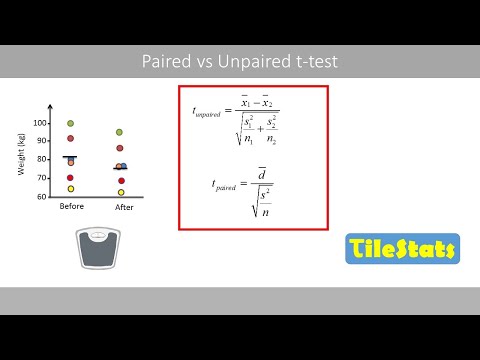
The paired sample t-test is to compare the means of two dependent or paired samples or groups. In general, it is used to compare the means before treatment and after treatment. You can watch the following video for the difference between paired sample t-test and unpaired sample t-tests.

▶️ Paired vs. Unpaired sample t-test

For example, we can test whether there is a difference in mean tcresult and tgresult. You can use two variables for paired t-test.

ttest var1 == var2

The output shows that the mean tcresult is 215.94, and the mean tgresult is 143.90. The difference is 72.04, which is statistically significant (p < 0.001). Further, you can see the observation size for the two variables are the same since they PAIRED for the sample that there are data points for BOTH VARIABLES.

Unpaired sample t-test

On the other hand, an unpaired sample t-test compares the mean for ALL DATA POINTS for each variable. Now, the observation size for tcresult is 10,351.

ttest var1 == var2, unpaired 

You can choose either paired or unpaired t-tests based on your data and research questions. To compare the means before and after the intervention (pretest vs. posttest), we are trying to see the change within each person, so using a paired sample t-test is recommended.

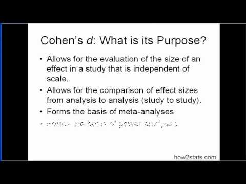
T-test with Cohen’s d Effect Size: esize twosample

Finally, we may want to report the effect size of the t-test, which measures how large or meaningful the difference between the means is. One common measure of effect size is Cohen’s d, which is calculated as:

To calculate Cohen’s d in Stata, we can use the esize twosample command with the cohensd option:

esize twosample var1, by(groupvar) cohensd

The output will show Cohen’s d for the difference in means of variable between groups. In the example, the effect size is -0.29, which is considered a small-medium effect size.

“A commonly used interpretation is to refer to effect sizes as small (d = 0.2), medium (d = 0.5), and large (d = 0.8) based on benchmarks suggested by Cohen (1988).” (reference: Lakens (2013))

To learn more about Cohen’s d, please find this video 🙌

Plot t-test: graph box

One of the best plotting methods for t-tests is a box plot! Please check out this post to see how to draw a box plot by group in Stata.

I hope this blog post was helpful for you to learn how to run t-test in Stata 🙂

References

How can I do a t-test with survey data? | Stata FAQ (ucla.edu)

Performing a Independent Means T-test in Stata – Stata Help – Reed College

Paired t-test in Stata – Procedure, output and interpretation of the output using a relevant example. (laerd.com)