[Stata] Comparing OLS and ML Estimation

Ordinary Least Squares (OLS) and Maximum Likelihood Estimation (MLE) are two ways to estimate relationships between variables in regression analysis.

OLS finds the best-fitting line by minimizing the squared differences between the actual values and the predicted values. It gives the most accurate estimates when certain assumptions hold, such as normally distributed errors and constant variance.

MLE, instead of minimizing squared differences, finds the estimates that make the observed data most likely. It assumes that the dependent variable follows a probability distribution and estimates the coefficients by maximizing the likelihood of seeing the given data.

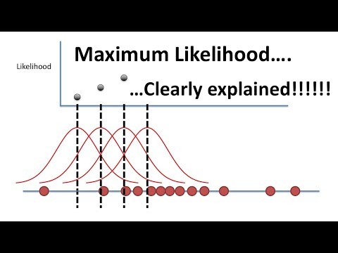
In simple cases, like linear regression with normal errors, OLS and MLE give almost the same results. However, MLE is more flexible and can be used when OLS assumptions don’t hold. The following video shows why maximum likelihood is invented:

Example

Let’s imagine you’re a researcher trying to understand how years of education affects annual income.

OLS (Ordinary Least Squares) Approach: Think of OLS like trying to draw the “best-fit” line through a scatter plot of education and income data. For each person in your study:

• Plot their years of education on the x-axis
• Plot their income on the y-axis
• Draw a line that minimizes the total squared distance between each person’s actual income and what the line predicts

For example, if someone with 16 years of education (bachelor’s degree) actually makes $60,000, but your line predicts they should make $55,000, there’s a $5,000 error. OLS squares this error ($25 million) and tries to minimize the sum of all such squared errors across your sample.

MLE (Maximum Likelihood Estimation) Approach: MLE takes a different perspective. Instead of minimizing errors, it asks: “What relationship between education and income would make our observed data most likely to occur?”

Going back to our example:

• MLE starts by assuming incomes follow a certain pattern (like a normal distribution) around the true education-income relationship
• For each possible relationship (line), it calculates the probability of seeing the actual incomes in your data
• It picks the relationship that makes your observed data most probable

So if you see someone with 16 years of education making $60,000:

• OLS asks: “How far is this from our prediction line?”
• MLE asks: “What education-income relationship would make this observation most likely?”

Key Differences:

1. If you assume income is normally distributed around your prediction line and has constant spread (variance), OLS and MLE will give you virtually identical results.
2. However, let’s say you notice that income spread increases with education (higher education leads to more variable incomes). In this case:
   • OLS might give misleading results because it assumes constant spread
   • MLE can handle this by explicitly modeling the changing spread, giving you more accurate estimates
3. Or perhaps income follows a different pattern, like being skewed (lots of lower incomes, fewer very high incomes). MLE can adapt to this pattern while OLS might struggle.

Stata Exercise

We will compare OLS and MLE by examining how age affects household size using data from Stata’s nhanes2 dataset. The model we estimate is:

housesize=Intercept+(Age Coefficient×Age)+error

The intercept tells us the estimated household size when age is zero, and the age coefficient tells us how much household size changes for each additional year of age.

To estimate the model using OLS, we use:

webuse nhanes2, clear
regress houssiz age

Running MLE in Stata

Instead of minimizing squared differences, MLE assumes household size follows a normal distribution and estimates the coefficients by maximizing the probability of observing the data.

We define the likelihood function in Stata:

* We need to create a program for our likelihood function
program define mlreg
    args lnf xb sigma
    quietly replace `lnf' = ln(normalden($ML_y1, `xb', exp(`sigma')))
end

Then, we estimate the coefficients using:

* Set up the ML estimation
ml model lf mlreg (xb: houssiz = age) (sigma:)
ml maximize

MLE gives us similar estimates to OLS but also reports the log-likelihood, which measures how well the model fits the data.

Both methods produce nearly the same intercept and age coefficient because our model assumes normally distributed errors. However, MLE also provides the log-likelihood, which allows us to compare different models more easily.

Visualizing the Results

We can create a scatter plot with the OLS regression line:

* Load NHANES2 dataset
webuse nhanes2, clear

* Run OLS
reg houssiz age
predict ols_pred

* Run MLE
program drop _all
program define mlreg
    args lnf xb sigma
    quietly replace `lnf' = ln(normalden($ML_y1, `xb', exp(`sigma')))
end

ml model lf mlreg (xb: houssiz = age) (sigma:)
ml maximize
predict mle_pred, equation(xb)

* Create three simple but informative plots
* 1. Basic comparison plot
twoway (scatter houssiz age, msize(small) mcolor(gray%30)) ///
       (line ols_pred age, sort lcolor(blue) lwidth(medthick)) ///
       (line mle_pred age, sort lcolor(red) lwidth(medthick)), ///
       legend(order(2 "OLS" 3 "MLE")) ///
       title("House Size by Age: OLS vs MLE Comparison") ///
       ytitle("House Size") xtitle("Age") ///
       name(g1, replace)

* 2. Residual plot
gen ols_resid = houssiz - ols_pred
gen mle_resid = houssiz - mle_pred

twoway (scatter ols_resid age, mcolor(blue%30)) ///
       (scatter mle_resid age, mcolor(red%30)) ///
       (lowess ols_resid age, lcolor(blue)) ///
       (lowess mle_resid age, lcolor(red)), ///
       legend(order(1 "OLS Residuals" 2 "MLE Residuals")) ///
       title("Residual Analysis") ///
       ytitle("Residuals") xtitle("Age") ///
       name(g2, replace)

* Combine graphs side by side
graph combine g1 g2, ///
    title("OLS vs MLE: Predictions and Residuals") ///
    rows(1) xsize(10) ysize(4)

Since OLS and MLE produce almost the same estimates, the two lines should be nearly identical.